xINvisionQ Case Studies
Introduction
The case studies displayed here include the scientific discovery of a freefalling light sphere trajectory and simulated Schrodinger's Cat thought experiment, a dataset from the M1 forecasting competition, and equity trading of the Dow Jones Index. This page will be updated regularly, as xINvisionQ can be run on all sorts of datasets including but not limited to the ones currently shown.
1. Scientific Discovery
Here 2 case studies of scientific discovery is presented; freefall of a light sphere and simulated Schrodinger's Cat thought experiment.
The freefall light sphere case study illustrates a classical, determined forecasting dataset: the trajectory of a freefalling light sphere is certain, with the initial conditions a function can be obtained to accurately reconstruct the past and map out its future trajectory. An important thing to note here is that since a light sphere is not a completely solid object, it's trajectory cannot simply be calculated by Galileo's free fall formula of h=1/2gt^2 since over the course of free falling the light sphere conforms differently to air resistance and gravitational acceleration. Thus the light sphere's freefall can't be calculated purely using calculus, making it a unique case study for forecasting.
For Schrodinger's cat thought experiment, we all know that the cat is "dead and alive simulataneously" but for the average Joe it doesn't really matter whether the cat inside the box is dead or alive. But for a observer who's a scientist, their natural instinct is to formulate hypothesis' and theories' to "predict" whether the cat inside is dead or alive before they open the box. And this is exactly what we can leverage, by using a simulated Schrodinger's cat thought experiment, we generate 25 boxes of cats set up in accordance to Schrodinger's original description (Geiger counter, radioactive substance, hydrocyanic acid), an observer or scientist then can open the first 19 boxes and see whether the cats' inside is alive or dead and then by studying the historical data of the previous 19 boxes of cats' they can then come up with predictions about the state of the remaining 6 cats', thus turning this into a decision-making under uncertainty problem, or in other words, a time series forecasting scenario.
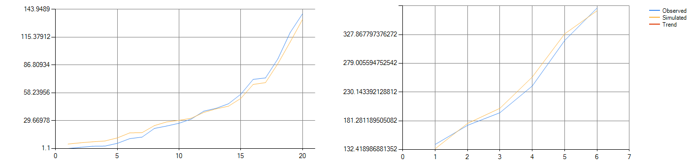 Figure 1-1: Freefall light sphere fitting (left) and forecast (right) graphs
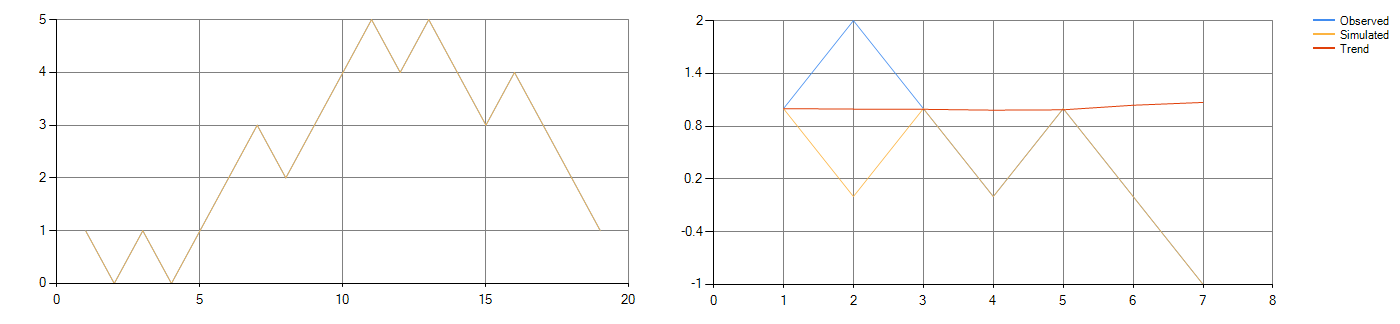 Figure 1-2: Simulated Schrodinger's Cat thought experiment fitting (left) and forecast (right) graphs
The graph on the left of figure 1-1 is the fitting graph of the freefalling light sphere, the graph on the right of figure 1-1 is the verify forecast graph of the freefall light sphere's predicted trajectory and its' actual future trajectory. The graph on the left of figure 1-2 is the fitting graph of the simulated Schrodinger's cat thought experiment, the graph on the right of figure 1-2 is the verify forecast graph of the following 6 boxes of cats' predicted state.
| Label | Calculated Distance | Original Distance |
|---|---|---|
| 21 | 133.756 | 141.0 |
| 22 | 176.798 | 173.5 |
| 23 | 202.488 | 195.0 |
| 24 | 255.784 | 240.5 |
| 25 | 329.132 | 317.8 |
| 26 | 368.132 | 373.0 |
Table 1-1: Verify forecast data values for freefall light sphere
| Label | Predicted Cats' State | Observed Cats' State |
|---|---|---|
| 20 | 1 | 0 |
| 21 | 1 | 1 |
| 22 | 1 | 1 |
| 23 | 0 | 0 |
| 24 | 1 | 1 |
| 25 | 1 | 1 |
Table 1-2: Action sequence for simulated Schrodinger's Cat thought experiment
Table 1-1 is the verify data of the freefall light sphere, the accuracy rate is 96%. Table 1-2 is the final action sequence produced to "guess" the state of the cats' in boxes 20-25, where 0 represents that the cat is alive and 1 represents that the cat is dead, and the prediction odds are 83%.
For more details, please read our paper AI Assistant Scientist: Aiding scientific discovery with quantum-like evolutionary algorithm.
2. M1 Forecasting competition
Here we present a case study of yearly dataset #T153 from the first M competition.
Given this dataset's unique nature, we are able to run both a classical and quantum forecast, fully highlighting xINvisionQ's dualistic forecasting abilities. Essentially, for the classical forecast, xINvisionQ can produce a function to fit its past trajectory and forecast its future trajectory; for the quantum forecast, xINvisionQ will utilize logic trees to fit its past and produce a probabilistic forecast.
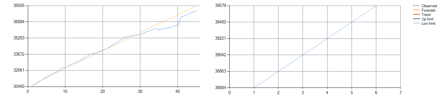 Figure 2-1: T153 classical fitting (left) and forecast (right) data
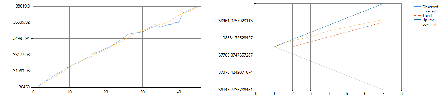 Figure 2-2: T153 quantum fitting (left) and forecast (right) data
As shown, the function produced by the classical train is linear, while the probabilistic forecast produced is non-linear. Figure 2-1 shows the linear fitting and forecast: the trained and predicted results are just a straight line. Figure 2-2 show the non-linear fitting and forecast: the fitting and prediction results fluctuate more.
In summary, if you just want to see an overall trend then a classical function linear analysis will suffice, if you want to see a more detailed approximate estimate then a quantum probabilistic non-linear analysis will do so.
This highlights the power and flexibility of xINvisionQ – one tool for all types of datasets.
3. Stock forecasting
In this case study presented, xINvisionQ studies the recent past of the market to find a trend, and by using the trend found to then produce a satisfactory forecast for the short horizon.
Figure 3-1 shows the training (on left) and validation forecast (on right) results. The blue line is the observed data, the yellow line is the data calculated by xINvisionQ, and the red line is the overall trend direction calculated.
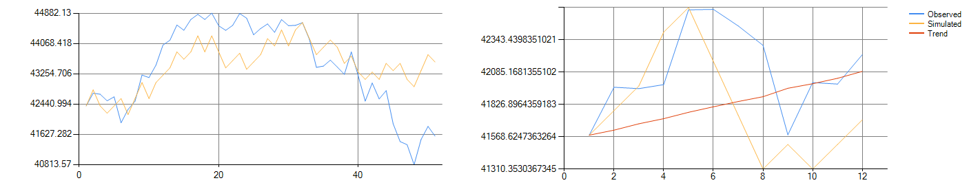 Figure 3-1: Dow Jones Index fitting (left) and forecast (right) data
4. Demo Videos
Below are the detailed videos of each case study dataset; videos here are not sped up for demonstration purposes, they are raw unedited footage.
Freefall light sphere:
Schrodinger's Cat thought experiment:
M1 Competition:
Dow Jones Index: