xINvisionQ Blog
Introduction
Welcome to xINvisionQ's blog!
Demystifying the double slit experiment
Is it a particle? Is it a wave? It's a randomly-jumping electron!
If one experiment captures the very mind-boggling, spooky, and elegant nature of the world we live in, none other than the single electron double slit experiment does better. Termed the central mystery of quantum mechanics and the most beautiful physics experiment, the experiment with "two holes" manifests the "counterintuitive" way a single electron, that is indeed a classical particle, can produce a wave-like diffraction pattern on a detection screen after being fired through either one slit or another. This strangeness has invoked many, if not absurd, interpretations, and the questioning of reality itself. Is it a particle? Or a wave? What about both? Maybe it goes through one slit in this world and the other in a parallel reality. But what if it's because we looked at it which caused it to suddenly become a particle? But wait, how would an electron know if we're "spying" on it? For 100 years this debate has raged on - starting from the very founding fathers of quantum mechanics in the "infamous" Bohr-Einstein debates. Bohr insisted that we shouldn't question what nature does and just accept it, in which he put forth his Complementary Principle - he even put the Yin Yang on his coat of arms to "prove" it. Heisenberg also echoed this, pointing to his Uncertainty Principle. But Einstein refuted that there must be something that we just don't know, something concealed from us that makes the final piece of the puzzle - an electron that's a physical particle just can't produce wave patterns under the very laws of physics, something must be missing. Schrodinger also blatantly agreed with Einstein as well (que his infamous cat). Whether you agree with Bohr or Einstein, what has also bothered many others is - if an electron is truly a particle why does it exhibit a wave-like interference pattern? How can an electron act like a wave when we don't know exactly which slit it went through but suddenly start to "fire" like a bullet when we detect which slit it went through? Well, we've dared to put forth a new way to think about it, one that's not counterintuitive - get ready to cast aside the whole wave-particle duality, it goes through slit A in this world and slit B in another world, and it's the "blinking of our eyes" that determines if it's a particle or a wave.
Drumroll please; and now for the big reveal - it randomly jumps! Well at least in our humble opinion. Think about it, there's been one thing that has been overlooked by default - everyone has assumed that an electron must move forward in a straight line like the firing of a bullet. But what if an electron randomly jumps around at will - once it parses the slit it zig zags through space and then lands at one specific point on the detection screen. And what causes these jumps is because of the step-length of each jump is so large relatively compared with the movement of a bullet - a bullet seems to fire in a fully continuous way but in fact it technically moves forward in "small steps" as time passes, except given its speed and cause the jumps are too small it can only fire in a continuous forward manner and can't move sideways. For an electron though, because it's step-length between movements is so much bigger it has the "leeway" to "change lanes" to produce the so-called illusionary wave-like pattern that is bestowed upon us. This way as it discretely traverses through the vacuum of space between the slits and the detection screen it can only be at some points and not everywhere all at once like a wave, therefore we see the "blobs" that make up the interference pattern, as illustrated perfectly by the experiments conducted - you can also see the "mysterious" wave-like pattern that we produced in our simulated experiment below.

According to our bold hypothesis, where we cast the whole counterintuitive, wave-particle duality out the window, we first firmly put forth that the electron is a particle and particle only - fundamentally it is no different than any other physical particle. We argue that there is no mind-boggling mysteriousness, each time an electron is fired from the starting source it randomly parses through either slit A or slit B, there is none of the going through both slits at once bogus, then it randomly jumps around that forms its uncertain trajectory, and then finally it lands on one specific spot on the detection screen, which forms the interference pattern. You can see the gradual build up of all individual electrons trajectories that we simulated in the figure below.
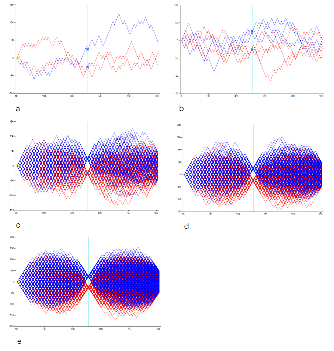
Finally as the build up of all the electrons marks on the detection screen form, we can see the 5 distinct "blobs" - where the white space in between are the places where none of the electrons landed because as the electrons jump they can only be at specific places and not everywhere. This "infamous" image can be seen from all the real world experiments conducted, as well as in our simulated experiment results below.
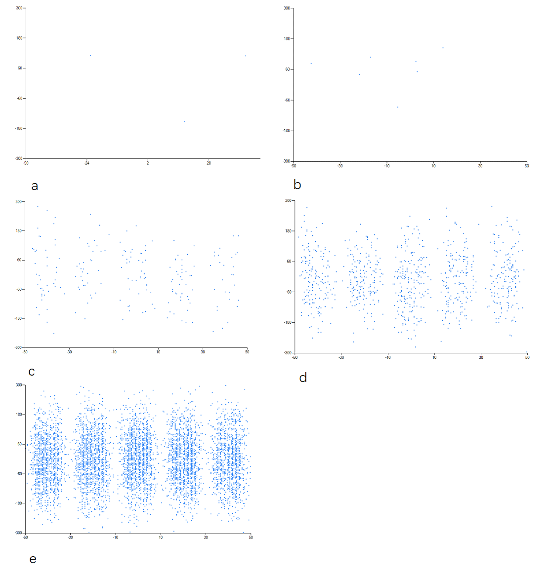
Whether from the trajectories of the electrons or the marks of where they landed we can see that when just a couple of electrons are fired through, both their trajectories and where they landed seem to be more uncertain and scattered, but with the gradual buildup of more and more electrons we see the more discerning interference pattern form. The intervals of the buildup we simulated were 3, 7, 196, 888, and 5975, in which their trajectories and marks correspond to a-e in the figures respectively. Therefore we can somewhat conclude that as the more electrons accumulate, they disperse and smear out across space, leading to the wave-like interference pattern all the while still being a physical particle. All the details of our entire methodology and hypothesis is beyond the scope for a single blog post, for more details, feel free to take a more deeper dive into our paper, On the Single Electron Double Slit Experiment - A Randomly-Jumping Electron Approach
Lastly, this whole conundrum, which has been debated for 100 years, arises from the electron's wave-like interference pattern, which has given rise to a plethora of interpretations and explanations like the sci-fi favorite Many Worlds where the electron passed through slit A in this world and slit B in another world, and QBISM where it puts forth that the electron passing through either slit is just a "figment" of our beliefs, and many more. Whether you believe in whichever one, I am not here to judge, but for those who prefer to stick with good ole' Copenhagen I leave you with if an electron can produce a wave-like pattern what about a shuttlecock? Could a badminton birdie be smashed through two gaps and randomly "jump" through the air and form a wave-like interference pattern? You better hope it won't land in Greenland.
A data analyst. An AI Assistant Scientist. An Induction Engine.
xINvisionQ’s INvisionary INnovation
Gazing above and peering within
“I think, therefore I am.” Or was “I dreaming of the butterfly or the butterfly dreaming of me?” The very nature of reality is just beyond what we can conceive, and as we tumble down the rabbit hole, philosophers like Descartes have argued that we should first doubt everything, then break down reality into the smallest bits possible and figure out the innerworkings of the smallest unit, and then piece them all back together to find the grand penultimate theory of nature and reality. However just thinking hard enough, or even thinking different will not lead us to discovering a unified theory of everything – when it comes to uncovering the mysteries of the universe “we must know, we will know” simply isn’t going to cut it.
Since the dawn of civilization, we have thrived to pull back the mysterious veil of mother nature, and to pinpoint the inner mechanism of the moral compass that guides us – the very two things that Kant alluded to – “two things awe me the most, the starry sky above me and the moral law within.” While peering above and within, we find ourselves in the face of a significant hurdle – the problem of induction. British Philosopher David Hume put forth this problem of induction, stating that induction alone is not enough for understanding the entire universe and predicting the future; because future simply can’t just be induced from past, whole from part, unknown form known. However, you’d be wrong to think that if pure induction won’t work, we could turn to deduction. Godel’s incompleteness theorems, or his proof, tell us that under an axotomized formal framework it’s impossible to prove theoretical hypothecation without correlating it with real empirical data.
We know now that when it comes to orchestrating nature’s grand symphony induction alone won’t work; pure deduction won’t either, cause quite frankly we’re not the conductor and have never been and won’t ever be. We humans have tended to put ourselves at the center of the universe, and we’ve formulated an induction-deduction methodology, induce what we can from experience, and then deduce the rest of the unknown. While this has served us well in some specific cases, as long as we find ourselves resident in this vast universe in which we cannot jump out of, we can’t find a “one-size-fits-all” grand solution.
Now, from the previous “revolutions” of Newton and quantum mechanics that upended our views of the universe, we hope to pioneer a paradigm shift – that’ll gain the most knowledge from nature, and it’s empirical and observed data. Thus, in order to truly “overcome” the limitations of our knowledge, our attention must be first diverted back to induction and deduction – however we do have a powerful “friend” to help us out a bit.
With the rise of computing, one in which we can’t help but wonder whether a machine could go about discovering the laws of nature. Throughout history, we have borne the brunt of thinking and with computer becoming more powerful, the words of Alan Turing start to become more relevant – “can machines think?” Could we get a machine to discover the laws of nature on its own, one that can work around the clock, and do its own conscious thinking?
A computer that we have now was merely a pipe dream in the days of Turing. One that could think was only limited to the imaginations and annals of science fiction. The advent of Artificial Intelligence now is like the impossible of when our ancestors looked up to the birds flying in the sky and could only sigh or wish that we humans could take to the skies as well.
Unfortunately, the current trend of AI, LLMs, and the world model are all the hype nowadays. Every big tech company is engaged in an “arms race” to build the next AI scientist, chatbot, or humanoid-like robot with an LLM or the so-called “world model”; however, the million-dollar question is how to overcome Hume’s problem of induction? Without a solution everything’s just self-hype – a bubble waiting to burst. Maybe we should ask ChatGPT how to do so; it’ll probably have no clue just like the companies that made it. The “big five” clearly don’t know how to implement a fundamental, generic induction engine to find regularities from any raw data, all without relying on any prior knowledge – the more may be merrier but the more data not so necessarily. Without an induction engine, just like how a car without a motor engine won’t make it out of your garage, AGI is merely a sweet dream – just keep sleeping. However, a solution to the induction problem is not Plato’s cave allegory, it’s more about striving for effective forecasts and not 100% accurate ones.
This is where xINvisionQ comes in. We strive to be that induction engine – one day you’ll say xINvisionQ it for all raw data just like how you say Google it today. We propose a metamorphic quantum leap from an induction – deduction approach to what we’ve termed a construction – evolution one. xINvisionQ as an induction engine, and more importantly acting in the capacity as a decision-machine will start off by constructing a population of formalized deductive models; then with three predefined inductive rules it’ll evaluate the performance of each model; finally, by utilizing an evolutionary algorithm, the best one will be optimized in a survival of the fittest faceoff style. Before that happens though, in the meantime if you do happen to be curious and ask ChatGPT, Gemini, Copilot, or DeepSeek “can you think?”, you might be just be greeted with “Of course I think, because I exist.”
What we do in a nutshell – The elevator pitch
This is exactly xINvisionQ does – a generic induction engine for getting the most valuable information and producing the most effective forecasts from any dataset: natural, social, economic, physical, any data. But xINvisionQ is more than just a search engine for data, it doesn’t brute force, blindly guess, or require vast amounts of prior knowledge but rather it finds regularities from all raw data semi-automatically by constantly self-adapting, self-learning, and self-evolving – strictly in three distinct parts. First, a formalized symbol framework is used to describe both nature’s (observed dataset) behavior and the induction engine’s corresponding “actions”; second, by following three predetermined inductive rules to evaluate the induction engine’s performance; and third, continually optimize the induction process with an evolutionary algorithm.
The Canvas and Brush – the xINvisionQ Model
Just like how looking up to the sky and putting down pure speculation in the form of observations will not lead us to discovering any scientific theories, attempting to getting the most important information out of pure raw data will not take us very far either. Thus, there needs to be a way of first describing raw data in a simple way for the induction engine to model and eventually find the most valuable information from it. This can be done by converting any dataset into a generic event series – based on its characteristics of up/down and the certain distance in between.
As Jim Al-Khalli wrote in The World According to Physics, “Everything that happens in the universe comes down to events that place somewhere in space and at some moment in time.”; therefore in the vast canvas of the universe we can “paint” everything that happens as an event taken by mother nature – in which “she” can “choose” to move up or down and any certain distance. Simply put, for any one-dimensional sequential dataset in general, there are two main characteristics – 1) either the succeeding point moves up or down relative to the preceding one; and 2) there is a certain distance that reflects the change of movement between the two successive points. Nature’s “behavior” is reflected by these movements; however, nature herself does not tend to laminate all the information regarding these characteristics beforehand. Without this crucial information, we are always painting catch-up, nature paints her majestic canvas and we can only follow suit – however with complete information we can paint what nature will paint beforehand: like how we can perfectly “paint” the freefall of an apple ahead-of-time. But most times, as nature waves her brush, we are more suited to “take” corresponding “actions” to counter “her strokes” – believe that nature will paint upwards or downwards and the certain distance between.
Again, ever since the start of civilization our thirst to know the exact intricate workings of the universe has never been quenched, our curiosity has pushed us to pull back mother nature’s mystery veil, her secrets shrouded in the dark. Now instead of pure speculation and wild-conspiracies of what exactly may be behind that veil, with the empirical observed data subtly transformed into an event series, we can get the induction engine take its best shot – but not like blindfolding our primate relatives throwing darts at a bullseye.
By describing the data as an event series based on its characteristics, we can then model it by invoking the mysteriousness of quantum mechanics; by superposing all the possibilities of nature’s movements and the corresponding “counter-movements” the induction engine can take with the superposition principle and the first three axioms of quantum mechanics all together under a unified complex Hilbert Space. The infinite possibilities of nature’s behavior of moving up or down and the corresponding actions of the induction engine believing nature will move up or down are woven into a superposition of up and down simultaneously because of the infinite probabilities that each up or down could be in, as reflected by its eigenstates, eigenvalues, and coefficients. With all of nature’s “behavior” describes by superposing its infinite possibilities, the induction engine can now simulate nature by take corresponding actions – either believing that nature will move up or move down.
Essentially before the induction engine “guesses” what nature will do, it’s also in a state of infinite superposition of believing up or down simultaneously, before the induction engine “makes up” its “mind” it’s in this state of both. The goal of the induction engine is to guess right each time to reconstruct the historical data and effectively predict the future data most effectively. It does this by parsing through the entire dataset and takes an “action” at every point; if the entire dataset is reconstructed according to this way, then the event series is modeled in a satisfactory way by the induction engine.
The Jury is out – Evaluation of the induction engine
Modeling is just half the story; anyone can claim anything, but in order to be actually good, it needs to be proven so – or innocent until guilty. Therefore, there needs to be an evaluation of the theoretical speculation or model; and to do so we must correlate speculation with empirical data.
The “jury” that’ll be doing the evaluating are three predetermined inductive rules – Similarity Degree (SD), Effective Operational Level (EOL), and Consistency. In conjunction, these three rules essentially all propel the induction engine to “guess” correctly every single time. SD is just how many correct guesses made over the total points in the dataset; EOL is then all the times it guessed correctly and with the greatest degree of belief according to the complex system of all the possible outcomes over the maximum returns of all the guesses; and finally consistency is just a simple comparison of the Mean Absolute Error (MAE) produced by the induction engine with the MAE of traditional statistical methods, where the induction engine’s MAE should be better than of traditional statistical methods.
While every model is evaluated in some way or another, the way we are evaluating the performance of the induction engine is to thrust it into a position to “overcome” or indirectly “bypass” Hume’s problem of induction; though in no way are we claiming to have “solved” it, no one can predict the future, but with the three inductive rules, the induction engine is in the best possible position to reconstruct the past and effectively predict the future.
With the inductive rules alone, the induction engine is able to “sidestep” the problem of induction and deduction, finding a middle ground in between; however, we can’t just arm the induction engine with a Russian roulette, it can’t just blindly guess and hope to come across some best way to effectively predict the future – a concern that Feynman had back in the day. Well to prevent this from happening, we’re going to turn our attention from the micro world of quantum superposition to one of the most spectacular and at times controversial phenomena of the natural macro world – evolution.
Not by pure chance or luck – Survival of the fittest model
When evolution is mentioned, what first comes to mind is probably Charles Darwin’s theory that says we evolved from monkeys. However, the applications of evolution are widely overlooked, and in our case, we can harness the very power and wonders of it to empower our induction engine. Just like how Feynman said that it would be impossible for a machine to come up with scientific theories on its own in his book The Character of Physical Law because it can’t just do so by blindly guessing, in which we 100% agree with, we would like humbly point out that he too may have underestimated the power of Darwinian evolution and natural selection.
In the most basic terms, everyone knows what natural selection is – the fittest individuals of a population survive long enough to pass their genes off to their offspring, while the rest are not “selected” for. In the biological world that would mean a butterfly that has a more leaf like pattern on its wings that gives is a more camouflage look will survive longer than one that doesn’t and after many generations almost all of the individuals in this butterfly species will most likely have this camouflaged trait. For the decision-machine, it needs to ensure that the “fittest” model survives, and what better than to draw upon the wonders of natural selection.
Now in order to get the best model without sheer brute force, pure luck, or have our primate relatives throw darts at a bullseye, brings us to another wonder of modern-day computing – Genetic programming (GP). GP, at its core is just an evolutionary algorithm, and for this algorithm to constantly refine and optimize the entire process it first generates a population of individuals, let’s say 300. Then it’ll calculate how “fit” each one is; after that it’ll apply some cosmetic (structural) change of crossover, mutation, and selection to each one as it pleases, and lines them all up according to how fit they are after the “surgery”. The “fitter” ones are now naturally chosen to be “parented”, passing along their outstanding genes to the “next generation”. The process then repeats; where offspring are “operated” on, lined up according to “fitness”, parented to produce the next generation, and so-on-and-so-forth.
This iterative generation after generation evolution, let’s say 80, the “fittest” model should hypothetically arise, and it’s the one that’ll be utilized by the induction engine. And this is exactly where the advantage lies – the more uncertain and complex environment it’s faced with the evolutionary algorithm has more of an advantage. Why so? Because the evolutionary algorithm balances exploration and utilization very well, it’s able to store already known existent knowledge (storing it as an entire population as a collective whole and not just for one single individual) as well as being able to build upon that already known information by utilizing crossover and mutation to explore even more valuable non-existent knowledge that’ll lead to better optimal solutions.
There also needs to an incentive; the decision-machine has to be rewarded for its correct guesses and punished for its wrong ones – otherwise there would be no “motivation” or the chance to “learn” from its mistakes for the decision-machine. Therefore, the evolutionary algorithm also reinforces a reward and punishment system according to the four possible outcomes of every “guess” made – being the decision-machine guesses right according to the direction of the dataset and it guesses wrong in the direction of the actual movement, and vice-versa. The more times its rewarded and less times its punished allows the decision-machine to accumulate the most experience, and also strengthen the evolutionary natural selection of the best model.
Essentially, the evolutionary algorithm constantly refine and optimize the entire process, from the induction engine starting out knowing nothing about nature or the dataset at all, to gradually discovering more and more in an iterative and incremental way, and more importantly throughout this continuous evolutionary refinement, the “fittest” model arises, which should be the one that consistently fulfills the preset threshold levels of the inductive rules – and also answering the call to Feynman’s greatest “concern”.
Event – Information – Operation: Lights. Camera. Action
At the end of the day, we are not trying to create a fully perfect, fail-proof machine that can accurately predict the future, but one that can self-learn, self-adapt, and self-evolve to “counterstrike” nature’s constant creative evolution – one that may cope with and even foresee the problems and solutions that eludes the designer of this machine. Data analysis shouldn’t just be about gathering the vastest amounts of data possible and finding a statistical average, scientific discovery shouldn’t just be about backtracking the past to predict the future, and induction shouldn’t just be about inferring whole from part, cause from effect, and unknown from known. We shouldn’t naively believe that nature is static and there is some simple elegant epitome structure of the universe and nature just “sitting” there waiting for us to discover, on our quest of finding more and more about the starry sky and moral conscience within it is indeed about discovering the unknown of the unknown, but more importantly it’s about challenging the uncertain, unpredictable, and modifiable human and mother nature.
From Chicago to the world – Where xINvisionQ will go
Since our founding in August 2024, xINvisionQ has gone from the lecture halls of academia conferences as an invited speaker at CEII 2025, onto the journals MDPI Entropy and Journal of Theoretical Economics and preprint platforms of Preprints and Jxiv, and to the acceptance of a premier startup visa program in East Asia and a renowned incubator in the Middle East. In the road ahead, we will continue to conduct our cutting-edge research on decision-making under uncertainty, time-series forecasting, and scientific discovery, best if possible in conjunction with the local and American universities located on the same premises as the incubator or within the greater city ecosystem in an Asian nation that’s been an innovation and technological powerhouse post WW2; tap into the resources provided by either program to scale xINvisionQ to the greatest degree possible; and to land corporate partnerships with fellow startups and established corporations with a local presence in each region as well. Whether it’s a university seeking the very fundamental laws of nature, or an industrial powerhouse corporation looking to enhance their AI research lab, xINvisionQ has the breadth to grow both from academia or commercially. No matter where xINvisionQ takes us, our INnovation will not be hampered – from Chicago to the world and beyond.
More than Data Analysis – to the starry sky and beyond
xINvisionQ sets out to revolutionize the data processing industry with three launches – a data analyst, an AI assistant scientist, and an induction engine. These also aren’t three different products either – they’re one, all with a three-layered approach of Model – Evaluate – Optimize. Got data? Need effective forecasts? Seeking out the laws of nature? xINvisionQ it.
From the shivering cold rinks to xINvisionQ, there’s been a quote that has always stuck with me, it hangs in the locker rooms of every ice rink in the world, said by the undisputed GOAT Wayne Gretzky: “I don’t skate where the puck is, I skate to where it is going to be.”; and at xINvisionQ we have attempted to do just that, and will continue to do that for as long as we can – to invision valuable information, to instigate efficient decisions, to inquire on the laws of nature, and to inspire all to embrace the uncertainty of our world when navigating through the complexity of data – all with one tool, any dataset.
Now if Kant were alive today, he would still say his two things, but he would add something at the end “three things awe me the most: the starry sky above me, the moral law within me, and the information around me.” Perhaps maybe even Einstein would change his mind and say, “indeed let’s not question whether “GOD” plays dice with the universe but rather question if we can play dice with “GOD”.”
Beyond the Random Walk - Searching for a uncertain market hypothesis
Part Three
What a roller coaster ride it’s been. If you’ve stuck with us till now, hopefully you’ve learned at least something – Brownian motion, the axioms of quantum mechanics, and superposition. Now in this part we’re going to address the second question of how do we make single-event forecasts of the market? Well, to try to do so we’ll need the help of another great scientific theory – Charles Darwin’s theory of Evolution (yes, evolution).
When answering the second question, keep in mind again that traditional economic theory says, “Hey the market is unpredictable, no one can predict it, so just don’t even bother trying.” They say that because it’s a perfect “cover-up excuse” for the inability of their statistical approaches that can’t produce single-event forecasts. For them to give you any type of prediction, first they’ll need a huge sample amount of data, and then they’ll tell you well for the past 100 years of the stock market it has evened out to a 50-50 random (well that’s not very useful for predicting tomorrow’s closing price) and two they’ll tell you that well 9999 out of 10000 times the stock market should “act” in this way but in reality what actually happens is the 1 outcome that technically shouldn’t have happened (this is why economic theory says that recessions only come about once in a blue moon, but in the real world they do so every couple of years). Instead of entirely equating the randomness of the market to Brownian motion, we’ve shown that the market is indeed uncertain, that it is the “interactions” between the traders’ and market that causes this dual-uncertainty, and that the informatively efficiency of the market of 50-50 is just a special case of the uncertain market hypothesis.
Now what we’ve done to attempt to predict the market, is one use a small sample of data to produce a short-horizon forecast (does a stock’s price 10 years ago really influence its price tomorrow?), and two we’ve “transformed” the forecasting process into a decision-making one. Essentially forecasting is a decision-making process, we don’t know what will happen in the future and so we make our best educated guess and try to guess right; for predicting the stock market that would mean to buy when the price increases and to sell when it decreases – and we’ve formulated an AI assistant agent to make the best “educated guess” but not blindly.
First, we define our agent and what it’s supposed to do: basically, buy when the price of the equity trends upwards and sell when the price of the equity trends downwards. Since there are only two possible actions (buy or sell, and they’re orthogonal) with a different degree of subjective probability (beliefs) for each one, thus we can very conveniently, just like how we superpose the equity’s price states of up and down, we can also “superpose” the actions that the agent can take as well. This superposed state of “mind” of simultaneously buy and sell is not actually a state where the agent can buy and sell at the same time, it’s just undecided in which specific action to take; just like when you decide to buy something or not, before you do so buy and sell are both options “superposed” in your mind. This observable operator (remember that any observable must be represented by a density operator under formalized “quantum-like” framework) can be stated in terms of Hilbert Space:

Where |a_1⟩⟨a_1| is buy and |a_2 ⟩⟨a_2| is sell; with the p_1 and p_2 being the subjective degree of beliefs that the agent has when it “decides” to buy or sell respectively. The third and fourth terms are a bit more interesting; they’re the “quantum interference” terms which indicate that the agent doesn’t know whether to buy or sell and sell or buy; these are all superposed together which creates the “all the infinite possibilities of buy and sell simultaneously.”
This density operator is directly observable, it’s just before the agent “makes its decision” the superposed state of buy and sell is still valid, making the decision is equivalent to a measurement and by doing so “collapses” the state to only one action of buy or sell with a corresponding degree of belief.
So now we’ve defined the agent’s “state of mind” before it makes a decision, the superposition of all the different possibilities that it can take, and now when it actually does “make up its mind”, when it “decides” to either buy or sell the superposed state “jumps” to one action with its corresponding degree of belief only, shown as:
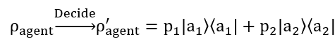
Where the “decide” can be seen as a “measurement” or “collapse” to one of the states. Now this is essentially just a projection or transformation from a pure state to a mixed state (pure state is the quantum superposed state, mixed state is the “collapsed” classical state, don’t get them mixed up), and it’s this decision process that is where the evolutionary algorithm does its “magic”. Essentially each “decision” the agent makes is the algorithm pitting each possible outcome against one another (survival of the fittest) and the potential increase or decrease of the stock’s price (the environment).
Now that we have agent defined, we need to know what the evolutionary algorithm does. The evolutionary algorithm is just an algorithm that’s based on Darwinian evolution in the real world, where it attempts to find the best of doing something through generations of mutation, crossover, and selection, just like how the fittest individuals of a population survive in a species, the same applies here.
In our case the evolutionary algorithm first randomly generates a population of possibilities (buy or sell with different degrees of belief), let’s say 300. Each of these individual possibilities are represented by a pure state which in turn is just an arbitrary 2x2 matrix, and because the density operator of the agent just so happens to be a 2x2 matrix as well, we can construct these density operators with the 8 most basic acknowledged quantum gates, which then leads the possibilities to become a “matrix tree”. Each one of these matrix trees represents an action of buy or sell with a said degree of belief that the agent can eventually end up using, with each decision made basically evaluating how effective or reliable each tree is, the fitter it is then it survives if not its discarded. Now how do we measure how effective each one is? Well, we need an evaluation metric; the four potential outcomes and corresponding actions that can be taken are the perfect way to evaluate how fit each one is. Since the price of a stock can only increase or decrease at any given time and the agent can choose to buy or sell, these four outcomes are: price increases and agent decides to buy, price increases and agent decides to sell, price decreases and agent decides to buy, and price decreases and agent decides to sell, resulting in this:
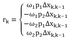
Where the first and fourth terms are that the agent makes the right prediction, and the middle two are the wrong ones. Therefore, we can naturally establish a reward-punishment system here for the evaluation metric; if the agent guesses correctly to what the price actually goes to then it is rewarded, if it’s wrong then a loss is incurred. This way when each possibility is evaluated the ones that are correct are kept and the ones that are wrong are eliminated, ensuring that the fittest ones survive. Now these four outcomes are just the expected values of each single decision made; the final fitness function is just the total (sum) of all the expected values of each decision made, which is this:

With the fitness function, the algorithm now takes each generated possibility and faces them off against each other, with the strongest knocking out the weaker ones, resulting in the one with the maximum fitness function to be used by the agent when making its final decision of whether the price will increase or decrease.
After generations of evolution, let’s say 80, the algorithm does its “magic” by putting each and every single possibility to the test and by the wonders of natural selection the fittest one survives and is used by the agent to make the final decision. With the goal of the agent being when the price is increasing to buy and when the price is decreasing to sell, therefore maximizing profit, and not just to buy and sell when the price is increasing or decreasing respectively but to do so with the greatest degree of beliefs. The goal is to buy with 100% degree of beliefs when the price is increasing, and sell with 100% degree of beliefs when the price is decreasing, but obviously to do so is much harder. But theoretically with the fittest possible actions that have been evolved by the algorithm and have stood the test of natural selection, it might be possible; if omega is 0.9, p is 100%, q is then increase, and a is to buy a strategy like this would be what the agent is aiming for, but most times this will not happen, so the next best thing to do is to attempt to predict the trend of the price, which we’ve illustrated in the results of our paper Is the Market Truly in a Random Walk? Now if we wanted to go further, we could take a shot at predicting the absolute closing price, because we’ve got the trend and if its right then we could potentially take a jab at the exact price. Well, that’s another blog post for another day. Meanwhile, maybe you could try to blindfold your cat and have it throw its toys at which stocks you want to buy.
Beyond the Random Walk - Searching for a uncertain market hypothesis
Part Two
By now it would be just be downright wrong to say that the market is not chaotic and random. While current economic theory agrees with that the market is random from all angles, whether from the markets or traders’ standpoint – with both viewpoints seeking to find the “invisible hand” that “guides” the market’s randomness. With EMH and of the current economic framework as an extension, the market or more importantly the stocks on the market are treated as the pollen randomly floating around in the petri dish, while the traders are considered the molecules around the pollen that are constantly colliding into them which causes the pollen to float around without a set motion, thus if the market is in a random walk the conclusion is that it’s unpredictable. However, as “critics” of EMH have pointed out that the market is not truly random: Robert Shiller has argued from a statistical standpoint that stocks don’t truly fluctuate randomly, as can be seen by “shocks” around the opening and closing bells as well as some breaking news; Daniel Kahneman argues from a cognitive psychology standpoint, he says that traders are not emotionless “molecules”, they are irrational and impulsive, with each and every trader’s behavior completely different.
However, regardless of what angle current economic theories tend to analyze the market from, they all run into two common problems – one though they all agree that the market and traders are inseparable and not in their own right, they can’t find a way to unifying describe both under one formalized framework; and two because they all depend on Law of Large Numbers, they need to make repeated observations of events in order to produce an average of it, thus this in turn makes it impossible for them to produce single-event forecasts.
Thus, this naturally begs two questions:
1) Could we model both the equities and traders all together as a collective whole?
2) Could we produce single-event forecasts of the market?
We will attempt to answer the first in this part; in the next and final part we will address the second question.
Unlike the abovementioned modern-day economic framework, where the market and traders are treated as randomly fluctuating entities, and that they can only be modeled separately, where stock prices act like pollen and traders are the molecules around it, and these elegant differential and diffusion equations can model their actions and behavior, the elephant in the room is that the market and traders’ are essentially inseparably intertwined or as we say “entangled” – it is the interactions between them that eventually “determines” the randomness, chaos, and uncertainty that has been symbolically known as the random walk. The elephant in the room is this dual-uncertainty: the market’s unpredictability “confuses” the traders, and all the traders’ “collective” actions cause the market to fluctuate and how to find an effective way to model both the traders and market all together under one formalized framework. Well, we’ve come up with this very subtle, shall we say ingenious way to do so – by calling on the principles of quantum mechanics, but not the actual physical sub-atomic formulation of it but just utilizing the mathematical linear algebra of it.
To do this we’ll be using the first three axioms of quantum mechanics. There are five axioms of quantum mechanics, however in our formulation we’ll only need to use the first three. Now, if you want you could go pick up a textbook and try to decipher what they mean; but if you don’t have a degree in quantum physics you might have a tough time understanding what they mean. I’ll save you the hassle and confusion and briefly go over them here.
The first three axioms are:
1. To every system corresponds a Hilbert Space H, whose vectors (state vectors, wave functions) completely describe the states of the system.
2. To every observable there is a corresponding unique self-adjoint operator A acting in H.

What the three axioms mean in plain English is actually quite simple, it’s not rocket science. The first axiom is that for anything in the quantum world, it can be described as a vector in Hilber Space, which is an abstract space that doesn’t exist in our 3D world, it’s purely in mathematical terms that we can’t see of feel. This state, and all the potential states that it can be in is denoted by the Greek letter Phi with Dirac bra-kets around it, |Ψ⟩, which represents that this is a quantum state. The second axiom is for every quantum state represented in terms of Hilbert Space there needs to be a density operator for it to be observed; and this second axiom is precisely one of the reasons that differentiates quantum mechanics from classical mechanics; because in classical mechanics you can define the state of something and observe it directly, but in quantum mechanics a quantum state as defined by axiom one cannot be observed directly, only its corresponding density operator can be observed, and axiom two defines the density operator for a quantum state which is represented by a Hermitian operator and all of its possible values of the state it can be in (its eigenvalues) are the possible values of the corresponding physical properties. The third axiom is the axiom of superposition and measurement – the uncertain state of a system can be expanded by its eigenstates that it could be in with a certain chance, thus all the possibilities are superposed, but you have to observe it to know which exact state it’s in, therefore once its measured, the uncertain state “collapses” to one of the prior possible states (eigenstates) with the probability of it being in that state is p(a_k)=|c_k |^2 (the absolute value of the coefficient squared).
With the basics of the axioms defined, we can use them to model both the market, or more importantly the trend of the equities price (up and down) and the actions that the traders can take (buy and sell). Before we do so, it’s important to note that we are not actually taking the physical properties of the closing prices of equities and the actions of buy and sell in the traders’ minds and “quantizing” them, we are merely utilizing the very nicely laid out mathematical linear formulation of quantum mechanics to model the many, infinite possibilities of the market and traders.
For the price of an equity (stocks, futures, bonds, treasuries, currency, etc.…) at a given time will either increase or decrease (it’ll either trend upwards or downwards), and at a given time a trader can choose to buy or sell; very conveniently we can superpose the trend of the equity’s price (increase or decrease) and the actions a trader can take (buy or sell), where we get:
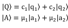
Where |Q⟩ is the superposed state of the equity’s price trend; and |A⟩ is the superposed state of the actions that can be taken by the traders. This superposition of states becomes very naturally convenient – a price of an equity either only trends upwards or downwards, while a trader can only take two actions of buy or sell, and these states are orthogonal, meaning they are polar opposites and only one can happen at a time. The trend of the equity’s price is represented by |Q⟩ where |q_1⟩ is increase and |q_2⟩ being decrease. c_1 and c_2 are the coefficients (the actual probability is then the absolute value squared of this coefficient). All the possible actions the traders can take are represented by |A⟩ where |a_1⟩ is the trader buys and |a_2⟩ is that the trader sells, and μ_1 and μ_2 are the coefficients (the actual probability is the absolute value then squared of it).
Superposing all the possibilities of the trend of the equity’s price and the traders’ actions may seem like a very nice way to express the inherent uncertainty – at any given time no one knows whether the price of an equity will trend upwards or downwards, and when traders are on the fence over whether to actually buy or sell. However just describing the superposed state of an equity and trader is not enough when trying to describe both as a collective whole, as they are “entangled”, this “entangled” state which is the complex system of all the superposed states is formulated as:
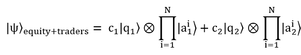
This complex system is where modeling both the equity and traders’ together under one framework is fully highlighted; here we have Phi with Dirac bra-kets
representing the entire state of the equity and all the traders, with the increase represented by |q_1⟩,
 representing all the traders
that decide to buy; with the decrease represented by |q_2 ⟩,
representing all the traders
that decide to buy; with the decrease represented by |q_2 ⟩,
 representing all the traders that decide to sell;
and the ⊗ being the
outer tensor product multiplying the two together. And this is exactly what results in the saying of how we are able to superpose all the possibilities of
increase and decrease as well as buy and sell; the coefficients could be any chance that the price increases, it could be 0.1, 0.5, 0.9, and it could even be
negative and that’s why its the absolute value squared that is the final probability or frequency of whether the price increases or decreases. Then we have all
the traders that buy when the price of this equity described is increasing, because this complex system only describes one equity on the market not the entire
market; and again
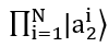
all the traders and the subjective probability (degree of beliefs)
that they have when they buy (because everyone will
have various degrees of confidence when they buy, thus resulting in the “infinite” possibilities of how many traders buy when this equity’s price increases),
then we have
which is all the traders the traders and the subjective probability (degree of beliefs) that they have when they sell.
representing all the traders that decide to sell;
and the ⊗ being the
outer tensor product multiplying the two together. And this is exactly what results in the saying of how we are able to superpose all the possibilities of
increase and decrease as well as buy and sell; the coefficients could be any chance that the price increases, it could be 0.1, 0.5, 0.9, and it could even be
negative and that’s why its the absolute value squared that is the final probability or frequency of whether the price increases or decreases. Then we have all
the traders that buy when the price of this equity described is increasing, because this complex system only describes one equity on the market not the entire
market; and again
all the traders and the subjective probability (degree of beliefs)
that they have when they buy (because everyone will
have various degrees of confidence when they buy, thus resulting in the “infinite” possibilities of how many traders buy when this equity’s price increases),
then we have
which is all the traders the traders and the subjective probability (degree of beliefs) that they have when they sell.
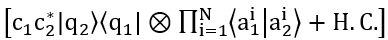
Now we have this elaborate way of describing both the possibilities of equity’s price trend and the traders’ actions, but we need to eventually validate this with the actual observed data. However, this complex system is not directly observable, it is only the vector describing the superposed state of the equity and traders’; in order to observe it we need to define a density operator according to the second axiom. This density operator is represented by:
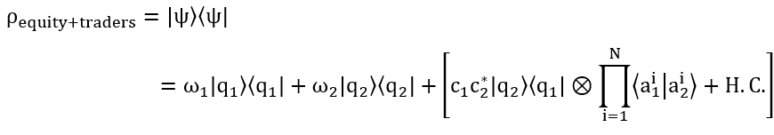
Where |ψ⟩⟨ψ| representing that this is a density operator, which also is a matrix, the first terms before the bracketed terms are just the two known states of the stock’s price (increase or decrease) and then the terms in the brackets are the “quantum interference” terms, where we don’t know whether the price will increase or decrease and whether all the traders will buy or sell, with H.C. being the Hermitian Conjugate.
These “interference” terms are precisely what illustrates the dual-uncertainty of the equity and traders – and how they “influence” each other through their “interactions”; q subscript 1 and subscript 2 are the price of the equity trending upwards and downwards respectively, and a subscript 1 and 2 are all the traders’ “collective” actions of buy and sell. This dual uncertainty arises like this: the price of an equity is inherently uncertain, we don’t know whether or not it’ll trend upwards or downwards in the next moment, so this “clouds” the traders’ decision-making abilities when they’re deciding whether to actually buy or sell; the first uncertainty of the equity influences the traders’ decisions and then the second uncertainty of the traders’ “collective effort” influences the equity’s price; the traders’ don’t know what the equity will “do” and the equity in turn doesn’t “know” what all the traders’ will eventually decide to do. But what we do know is that we can map the two “extremes” – when all the traders decide to buy or sell at the same time, which is highly unlikely but if so then the price of the equity will 100% surely go up or down respectively, and that when there are a near-infinite number of traders all buying and selling “randomly” (a lot buy and a lot sell), the price of that equity will indeed “act” how EMH says in a 50-50 random walk.
When there are infinite number of traders the price of the equity will start to behave as stated by EMH, but under the umbrella of our uncertain market hypothesis, this is just one certain special case – most times it is indeed in a random walk, but just like in the real world the I told you so only works on an average of times not every time. With a lot of traders trading an equity, it’s “behavior” will start to look something like this:
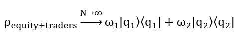
Because the “interference” of
 from above is now “cleared” because when N→∞ this
 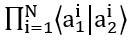 is now 0; where ω_1 is the objective frequency (probability) that the entire market will go up and ω_2 is the probability of decrease.
Most times ω_1 and ω_2 will be both equal to 0.5 or 50-50 which would show the market is in a random walk, but sometimes, in the real world this frequency won’t always equal 50. This happens because when there are so many traders’ buying and selling at one time they will “cancel” each other out – i.e. around a million traders’ buy which causes a slight uptick in the price of the equity but then also around a million traders’ sell which then pulls the price of the equity down again, thus the end effect is that the price of that equity then hovers around 50-50. However, on some occasions, out of the many traders actively trading, more are buying or more are selling thus this could lead ω_1 and ω_2 to be 0.3 and 0.7, 0.55 and 0.45, or even 0.01 and 0.99, which causes the equity’s price too not be in such a evenly random fluctuation, eluding to what was stated earlier with around the opening/closing bells and other external news “shocks”; this shows that the market is random but more importantly uncertain because once a equity is listed on the market it only “comes alive” once traders start trading it, but once that happens it’s price starts to fluctuate, and when it does traders aren’t 100% sure whether to buy or sell, and then once they do in turn it is the “collective effort” of all of the participating traders and they actions that then “determines” the closing prices of equities on the market – in this never-ending constant cycle of dual uncertainty – in which we shouldn’t just naively and stubbornly equate the prices of equities and the actions of traders to the randomly floating pollen and molecules in a petri dish, ones that can be described by a diffusion equation (although that diffusion equation was formulated by someone who’s name is synonymous with genius).
Now that we’ve shown how to model both the market (equities) and traders as a collective whole under one framework, and that the random walk is in fact just a special case of our uncertain market hypothesis, on to the million-dollar question, which was alluded to earlier, now becomes how do we make single-event forecasts of the market?
Beyond the Random Walk - Searching for a uncertain market hypothesis
Part One
What do pollen randomly floating around in a petri dish and stocks on the stock market have in common? At first glance the two may seem completely unrelated, and it might seem crazy to equate traders in suits crammed on the trading floor yelling at which stocks to buy with mad scientists in lab coats peering at pollen in a petri dish through microscopes. However, at a deeper glance, the one thing that the two share in common is their randomness – which is exactly what struck two of the greatest minds in science when seeking to find a way to describe the randomness of pollen floating around in the petri dish and on the stock prices on the market.
This phenomena of randomness has come to be known as Brownian motion, named after the Scottish botanist Robert Brown, who in 1827 described the way of pollen randomly floating around or fluctuating when he was looking at pollen grain under a microscope, however he did not describe what exactly causes the random movement of the pollen to happen – it wouldn’t be until around 80 years later that Robert Brown’s “accidental” discovery would led to the formulation of our understanding of the atomic world and the stock market; one could even go to call Brownian motion to be the “first” hypothesis to unify both the natural and social sciences – and this would be credited to two then-young Europeans, Louis Bachelier and Albert Einstein.
Einstein’s original mission was to “prove” that there are subatomic molecules or atoms that collide with the pollen and continually bump and crash into them to cause the pollen to randomly float around in liquid or a petri dish, and in doing so “overturned” the long-held belief that nothing exists beyond what we cannot see. Bachelier on the other hand, saw the randomness and immediately drew parallels with the stocks fluctuating on the stock market, one that he would use the concept of Brownian motion to describe how stocks on the Paris Stock Exchange randomly fluctuate just like pollen does in a petri dish, which was the topic of his dissertation The Theory of Speculation that he wrote in 1900 five years before Einstein’s seminal paper – and that is exactly why any social scientist will humbly point out that Bachelier was the first to describe Brownian motion, but most only remember Einstein, one because he put forth a more systematical mathematical approach, but two more so because his name is synonymous with genius.
Regardless of which original mission Brownian motion was applied to, in the simplest terms Brownian motion states any particle that is submersed by molecules around it, these molecules will collide with the particle in question, or pollen as originally observed, and in this case the exact precise location of where these particles will end up cannot be accurately calculated – only a probability of where they might be can. Brownian motion tells us that we can’t calculate the exact precise trajectory of where the pollen will end up, or diffuse to, unlike how we can for a freefalling apple.
Thus, this is where Einstein came in and gave a radical new interpretation by obtaining the new partial differential equation:
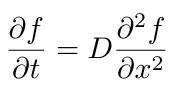
Where D is the diffusion coefficient.
Using this diffusion equation, we can then calculate the probability of where a particle of pollen will end up after a given time. This uncertainty of not being able to calculate a precise trajectory is because there are so many molecules surrounding the pollen and they can “bump” into them in all directions and its practically impossible to calculate which molecule will bump into it from which direction, but also more importantly because there are so many molecules surrounding it we can’t know the initial conditions of each and every one, but theoretically if one day someone is able to develop a supercomputer to calculate the exact movement, position, speed, and velocity of the molecules around the pollen then technically you could find exactly where the pollen will end up – but that is not the main point here, the point is that "the displacement of the suspended particles can then be described by a probability distribution that determines the number of particles displaced by a certain distance in each time interval" (Ann. Phys. (Leipzig) 14, Supplement, 23–37 (2005)), given that the motions of the particles are mutually independent of each other.
As with Einstein’s explanation, Louis Bachelier also agreed and stated that Brownian motion is a stochastic process – one that is perfect for describing random fluctuations. However, unlike Einstein, Bachelier didn’t really bother about proving that there are atoms “bumping” the pollen around, instead Bachelier saw the parallels between the randomly floating pollen as stocks “floating” up and down on the stock market and the traders as the molecules around it that “bump” them to go up and down through their actions of buying and selling. Thus, Bachelier took this metaphor and formulated a stochastic model of how stocks fluctuate on the market just like how pollen does so in a petri dish, stating that by using the partial differential equation doesn’t allow us to find the absolute price of a stock but a probability of what it might be or whether it will go up or down can be done so though. By doing so, Bachelier showed that a physical process such as Brownian motion can be used to describe the stock market, and his formulation would lead to the current most-well known theory of the market.
Building off of the concept that the market is in a random walk, Eugune Fama would put forth the Efficient Market Hypothesis, one that states that markets are informatively efficient, and that all the information of a stock is reflected in its current price – drawing off the implication of the Brownian motion random walk metaphor (assuming that the market is indeed truly in a random walk). Since EMH states and presumes that the market is completely random this also comes with the acknowledgement that no one can predict the market, because its already “informatively efficient”, and that all the stocks and traders are mutually independent of each other just like how the motions of the pollen are as well. This leads to some “counterstrikes” right away, one the market is uncertain because of the traders involved – it is the traders buying and selling that causes stocks to fluctuate, and two these participating traders are living human beings – ones with emotions and at most times irrational impulses when trading, with two of the major “opponents” of EMH being Robert Shiller who argues that the market is not always completely random from a mathematical and statistical standpoint and Daniel Kahneman who argues from traders' standpoint that these traders tend to exhibit unexplainable behaviors when trading.
Thus, for the time being, Brownian motion is the go-to explanation of anything random, be it pollen that randomly floats around, stocks that randomly fluctuate because of traders buying and selling, or a drunk person making their way home after a long night at the bar due to the colliding of “beer” molecules that they just indulged in colliding with the neurons in the brain, Brownian motion also shows us that pure randomness does not equate to uncertainty, something that we attempt to show with our formulation of an uncertain market hypothesis, one that agrees with the Efficient Market Hypothesis and Brownian motion that the market is indeed random, but more importantly uncertain – because of the “interactions” between the “entangled” traders and market.
Quantum Mechanics' Centennial - The first 100 year evolution of an unfinished revolution
Updated on September 25th, 2025.
Quantum mechanics celebrates its "100th birthday" in 2025 - and in honor of one of the most disruptive theories we've ever discovered, we take a look at journey of quantum mechanics and its story. Here's to the past 100 years and the next.
Throughout human history there have been a few times where our entire perspective on the very nature of reality has been changed. The Copernican revolution gave us a home, one that albeit put us on a spec rotating our Sun and not the other way around in the vast galactical cosmos. The Darwinian revolution gave us a family, one that told us that our chimpanzee relatives and all living species on our planet share the same common ancestor as us. One of the more recent revolutions, and one of the more important revolutionary paradigm shifts celebrates its centenary which the United Nations has dubbed the International Year of Quantum Science and Technology.
While the quantum story starts in 1900 when Max Planck discovered that energy is released in discrete packets called quanta, the quantum “revolution” started, if we were to pinpoint one place and time to mark the “true” inauguration of quantum mechanics, on the wee hours of June 1925, when Werner Heisenberg, an aspiring, young physics postdoc, at the tender age of only 23 and relatively unknown at the time would, as the story goes, climbed atop a boulder on the tiny 1 km2 island of Heligoland off the northern coast of Germany and elegantly gleam at what we now know as matrix mechanics, the first formal mathematical formulation of the physics that started off messy and took a quarter decade to mature, one that completely disrupted our views of the world and put into light how mother nature seemed to play dice with the universe as we know it.
With Heisenberg’s formulation of matrix mechanics, a whole spectrum of unresolved “questions” has been laid to earth. A cat that can be dead and alive at the same time. Is something a wave, or is it a particle? How can it be both? A “particle” (electron) that can go through two slits at once. Two “particles” the universe apart can someone “know” the state of the other one that leads to “Spooky action at a distance”. “God plays dice with the universe.” It’s we the observer, or more precisely how we measure something that leads to a collapse to either one state or another. An electron that can teleport through walls. And if you want to know the precise location of an electron you won’t be able to know its momentum.
While our grasp of quantum mechanics has given rise to unimaginable technologies, such as the lasers that store our precious memories on DVDs and blaze information through the ethernet cables of the Internet, the microchips that power our smartphones and laptops, help generate non-invasive images of the human body with MRI machines, and powering our GPS signals, as well as leading to the emerging vision of quantum computing, we indeed owe a lot to quantum mechanics. But we are still quite some ways from the ultimate pinnacle on the quest to truly understand the scientific and philosophical implications of quantum mechanics. It isn’t rocket science, it’s quantum mechanics.
While ever since Issac Newton formulated classical mechanics, up until quantum mechanics arrived on the scene, classical mechanics has done the job quite well, if not perfectly. Newton has told us that the planets orbit the Sun in the same way as how an apple falls from a tree. Basically, with the initial preconditions of something, we can with 100% accuracy calculate where it will end up. But in quantum mechanics, things aren’t quite that simple. In classical mechanics, if you’re sloppy, or if you have a broken-down ruler, you might get slightly different measurement readings once or twice, but that doesn’t change the length or height of whatever you’re measuring. Just like when you measure your height you might get 6”1’, while your uncle Joe might only get a reading of 5”10’, and when you go to your doctor for a physical, they might tell you that you’re in fact 5”11’, but nonetheless that doesn’t physically change how tall you are; you’re 5”11’ no matter what. But according to quantum mechanics, as a metaphor, you could be 6”3’ one time, 5”2’ another, and maybe only 1 inch tall some other time, because it is the act of measuring that causes your “height” to be determined, and this is the biggest difference the deterministic elegant classical mechanics, and the mind-boggling chaotic quantum mechanics. The main difference is that because as of now all measuring devices are macroscopic in size and follow the laws of classical mechanics; for classical objects that are being measured they’re the same size in scale of the measuring instrument, thus the measuring instrument doesn’t “disrupt” the object being measured. But for objects at the quantum scale, the measuring instrument will “disturb” the object being measured which causes the result to be uncertain. And this is precisely the problem when it comes to quantum mechanics, the question is where is the boundary between classical and quantum? When does something act in accordance with the classical mechanics formulated by Newton at the macro level and when does it start to be governed by the microscopic quantum laws? This question has puzzled physicists for the past 100 years, and very likely this it will continue to do so.
Over the course of the first century of quantum mechanics, many tend to overlook the statement by Richard Feynman, who once said, “I think I can safely say that no one understands quantum mechanics.” Well, it’s safe to say that after 100 years still no one really understands quantum mechanics. And many have probably forgotten the heated debates between Bohr and Einstein on the fabric of reality, where Einstein stubbornly insisted that “God” does not play dice with the universe and Bohr pessimistically saying that we shouldn’t tell “God” what to do and just “give into” nature because of its complementary manner. The main reason why the whole debate over what quantum mechanics fundamentally is has been so persistently heated to this very day is because quantum mechanics is essentially counterintuitive; and it is because of how bizarre quantum mechanics seems that has given rise to many different if not even more head-scratching interpretations of the matter, with three major ones: Copenhagen, many-worlds, and QBISM.
The Copenhagen interpretation, pioneered by Niels Bohr and Werner Heisenberg, is the major interpretation of quantum mechanics that is still widely taught in textbooks. Essentially Copenhagen is synonymous with uncertainty, complementing Bohr’s correspondence principle and Heisenberg’s uncertainty principle. Copenhagen’s major insistence is that something is only real once it’s measured; before it’s measured, even though it can be perfectly described by the Schrodinger equation no one can be sure what it is exactly – but only after it is measured it can exist in all possible states. With Bohr and Heisenberg being firm believers in the Copenhagen camp, the Copenhagen interpretation tells us that we should not be discussing whether or not something actually exists but how to describe it after we can observe it. In the case of Schrodinger’s cat, which was originally formulated by Schrodinger to show that quantum mechanics is incomplete and as a rebuttal to Copenhagen, but nonetheless Copenhagen says that his cat is “dead and alive simultaneously” until someone opens the box and looks.
The many-worlds interpretation is the most sci-fi friendly interpretation, and it has been the subject of many movies and TV shows. Many-worlds, or parallel worlds, leaves more to the imagination; you’re hard at work here in this world while you might be relaxing on a beach in another. Though while its original proposer, Hugh Everett did not intend for it to be a silver screen hit interpretation of quantum mechanics, the fundamental idea of many-worlds is that with every measurement the universe “splits” into parallel existing realities. Essentially all the possible states of something exists in other parallel worlds, when we observe something, we only see one possibility while all the other possibilities cease to exist here but continue in some form or another in a parallel time and space – one in which we can’t “communicate” with. Along the lines of this logic, then essentially, we can say that Schrodinger’s poor cat is alive here in this world and unfortunately met its demise in another.
Lastly, QBISM also a radical interpretation in its own might, saying that is our subjective beliefs, prior and posterior that help shape the very reality of our world. QBISM states that the quantum mysteriousness is just a reflection of our subjective understanding and interactions with the subatomic quantum world, and attempts to put the observer or scientist back into science. QBISM states that it is the beliefs we formulate and the new information that we constantly obtain to update our beliefs which leads to what’s being observed to be in the state that it is in, just like how our feline friend locked in the box is either alive or dead.
Heisenberg is also known for his Uncertainty Principle that tells us if you know where a particle is then you can’t know it’s momentum and vice versa. From an information perspective if we want to know more about something then we have to “sacrifice” knowing less about another, and though frustrating, unfortunately nature tends to never give us complete information. As Heisenberg said, “What we observe is not nature itself, but nature exposed to our method of questioning.” In the 100 years since, we have seen that mother nature seems to not play “her” cards in conventional ways, and “God” seems to play dice with the universe.
Now here's to the next 100 years: whether or not our descendants will still be asking does “God” really play dice with the universe or have found an answer to if we can play dice with “God”; maybe when we’re long gone, they’ll look back at us and say amongst the then current Einstein’s, Bohr’s, and Heisenberg’s – how in the world did our ancestors believe in quantum mechanics? But maybe, just maybe nature itself doesn’t “adapt” to anyone or anything, it’s constantly evolving and never has been set in stone for anyone to find its deepest secrets, and in 100 years, 200 years, or 1000 years, no matter what it’ll still be humankind adapting to nature and not the other way around.